Phase space
Consider a one-dimensional harmonic oscillator evolving according to the equation of motion:
\[m \ddot{x} + kx = 0\]It is possible to investigate the essential properties of \(x \left( t \right)\) using a geometric intuition solely by playing with the equation of motion, rather than directly finding the general solution analytically.
Firstly, for future ease, we define a parameter \(\omega = \sqrt{\frac{k}{m}}\). Performing this substitution in the equation of motion and dividing both sides by \(\sqrt{mk}\), we find,
\[\omega^{-1} \ddot{x} + \omega x = 0\]Now, we define a new coordinate \(y\) such that,
\[y = \omega^{-1} \dot{x}\]Substituting \(\ddot{x} = \omega \dot{y}\) in the equation of motion, we have,
\[x = - \omega^{-1} \dot{y}\]The space characterized by \(\left( x, y \right)\) is known as phase space. We imagine a system to trace a trajectory in its phase space through its evolution. The components of the velocity vector concerned are precisely given by the two above equations. Written in vector form,
\[\begin{pmatrix} \dot{x} \\ \dot{y} \end{pmatrix} = \omega \begin{pmatrix} y \\ - x \end{pmatrix}\]Therefore, we have transformed the original equation of motion, a one-dimensional second-order differential equation to a two-dimensional first-order differential equation.
Velocity vector field
The state of a system at any instant is given by the position vector:
\[\pmb{r} = \begin{pmatrix} x \\ y \end{pmatrix}\]The interesting thing about the vector equation of motion is that the velocity vector \(\dot{\pmb{r}}\) obtained from it is always perpendicular to the position vector \(\pmb{r}\),
\[\begin{aligned} \dot{\pmb{r}} \cdot \pmb{r} & = \dot{x} x + \dot{y} y \\ & = \omega y \: x - \omega x \: y \\ & = 0 \end{aligned}\]The second important feature is that for constant \(r = \lvert \pmb{r} \rvert\), the magnitude of velocity \(u = \lvert \dot{\pmb{r}} \rvert\) is also constant:
\[\begin{aligned} u & = \sqrt{\dot{x}^2 + \dot{y}^2} \\ & = \sqrt{\omega^2 y^2 + \omega^2 x^2} \\ & = \sqrt{\omega^2 \left( x^2 + y^2 \right)} \\ & = \sqrt{\omega^2 r^2} \\ & = \omega r \end{aligned}\]The only motion where the velocity vector is perpendicular to the position vector is that of circular motion about the origin. Furthermore, since \(u\) is constant for a given radius \(r\), the speed of revolution about the origin is also constant along a given trajectory.
Therefore, all possible trajectories of harmonic oscillators in phase space form concentric circles. The velocity vectors are tangential to these circles, and together for all circles, form a velocity vector field resembling the below:
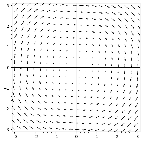 Velocity vector field
For readers who might be interested, the above plot can be generated in SageMathCell using the Sage code below:
1
2
3
x, y = var('x y')
plot = plot_vector_field((y, -x), (x,-3,3), (y,-3,3))
plot.show(aspect_ratio=1)
(Here, we have used \(\omega = 1\) for simplicity of the code).
Solution
Merry-go-round
Due to the circular symmetry of the velocity vector field, we can reduce the two-dimensional equation of motion to a one-dimensional problem, while still keeping it first-order.
To do so, we will use the \(r\) coordinate used earlier, \(r = \sqrt{x^2 + y^2}\) and define a new coordinate \(\theta\) such that,
\[\begin{aligned} x & = r \cos \theta \\ y & = r \sin \theta \end{aligned}\]Before proceeding to write the vector equation of motion in terms of these new variables, let us prove that for a given trajectory, \(\dot{r} = 0\). This will reinforce the idea that a given \(r\) characterizes a single trajectory (since it remains constant throughout).
Recall that \(u = \lvert \dot{\pmb{r}} \rvert\) is given by \(u = \omega r\). Therefore,
\[\dot{r} = \omega^{-1} \dot{u}\]Now,
\[\begin{aligned} \frac{d}{dt} \left( \pmb{r} \cdot \pmb{r} \right) & = 2 \dot{\pmb{r}} \cdot \pmb{r} \\ \frac{d}{dt} \left( r^2 \right) & = 2 \dot{\pmb{r}} \cdot \pmb{r} \end{aligned}\]But we know that \(\dot{\pmb{r}} \cdot \pmb{r} = 0\). So,
\[\begin{aligned} \frac{d}{dt} \left( r^2 \right) & = 0 \\ 2 r \dot{r} = 0 \end{aligned}\]Since \(r\) is arbitrary, \(\dot{r} = 0\).
In the phase space characterized by \(\left( r, \theta \right)\), this is an equation of motion, i.e. \(\dot{r} = 0\). It tells us that for a given trajectory, \(r\) is constant, which justifies the claim that each trajectory is in turn described by some \(r\).
But \(\dot{r} = 0\) doesn’t tell us much as an equation of motion. We are yet to compute \(\dot{\theta}\), which will give us a second equation of motion, and with more information about the evolution of the harmonic oscillator. This is why we said that we are reducing the two-dimensional problem to a one-dimensional one.
Equations of motion
Equipped with the knowledge that \(\dot{r} = 0\), let us recall the original vector equation of motion and use the \(\theta\) coordinate defined earlier:
\[\begin{aligned} \frac{d}{dt} \begin{pmatrix} x \\ y \end{pmatrix} = \omega \begin{pmatrix} y \\ - x \end{pmatrix} \\ \frac{d}{dt} \begin{pmatrix} r \cos \theta \\ r \sin \theta \end{pmatrix} = \omega \begin{pmatrix} r \sin \theta \\ - r \cos \theta \end{pmatrix} \end{aligned}\]Since \(\dot{r} = 0\), we can bring out \(r\) from the derivative and cancel it out on both sides,
\[\begin{aligned} \frac{d}{dt} \begin{pmatrix} \cos \theta \\ \sin \theta \end{pmatrix} = \omega \begin{pmatrix} \sin \theta \\ - \cos \theta \end{pmatrix} \\ \dot{\theta} \begin{pmatrix} - \sin \theta \\ \cos \theta \end{pmatrix} = \omega \begin{pmatrix} \sin \theta \\ - \cos \theta \end{pmatrix} \\ \dot{\theta} \begin{pmatrix} - 1 \\ 1 \end{pmatrix} = \omega \begin{pmatrix} 1 \\ - 1 \end{pmatrix} \\ \begin{pmatrix} - \dot{\theta} \\ \dot{\theta} \end{pmatrix} = \begin{pmatrix} \omega \\ - \omega \end{pmatrix} \end{aligned}\]The two equations above are really telling the same thing: \(\dot{\theta} = - \omega\). The solution of this equation of motion is trivial:
\[\theta \left( t \right) = \theta_0 - \omega t\]where \(\theta_0\) is a constant. Likewise,
\[r \left( t \right) = r_0\]Thus, a given trajectory of radius \(r_0\) resembles circular motion about the origin with frequency \(\frac{\omega}{2 \pi}\). Since each point in the phase space encodes the state of the system, this means that the harmonic oscillator itself displaces in this periodic fashion. The original \(x\) coordinate encodes this displacement, so \(x \left( t \right)\) must be some periodic function. Furthermore, as \(x\) is a projection of \(r\) onto the \(x\) axis in phase space, \(x \left( t \right)\) must be a projection of circular motion, i.e. sinusoidal.
Conclusion
After all our substitutions and tricks, what we have learnt is that \(x \left( t \right)\) is sinusoidal for a harmonic oscillator. We did so without explicitly finding \(x \left( t \right)\). Instead, we tracked the evolution of the system in phase space, and solved for more convenient coordinates \(r \left( t \right)\) and \(\theta \left( t \right)\).